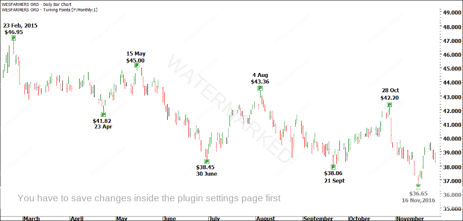
Your job was to run Geometric Angles from each of the starting points shown in Chart 1 below. They are the start and end of each big picture section.
Chart 1
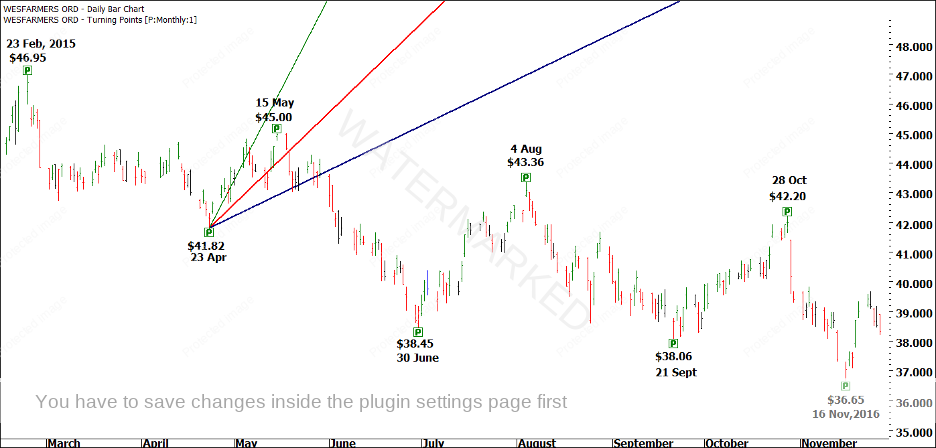
First, the obvious one is to apply your angles to the major high of 23 February, 2015, as shown in Chart 2, below.
Chart 2
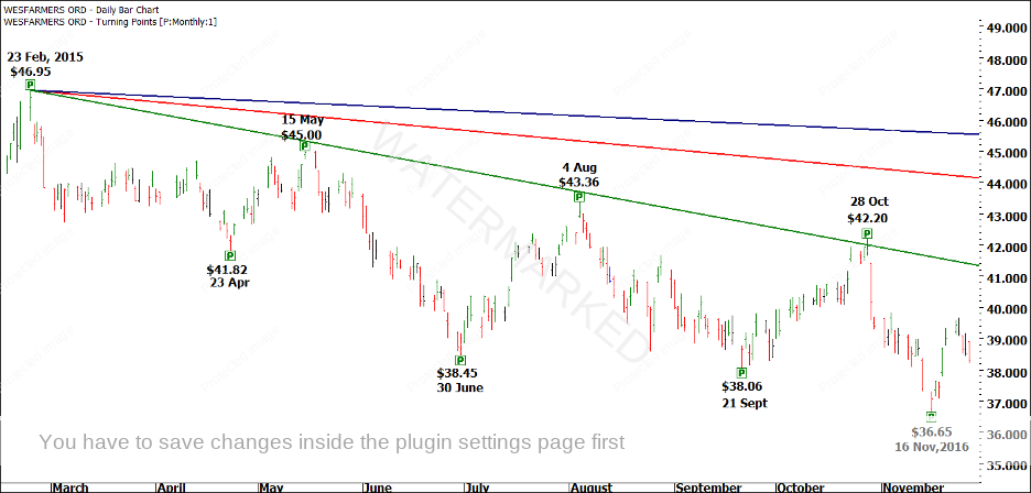
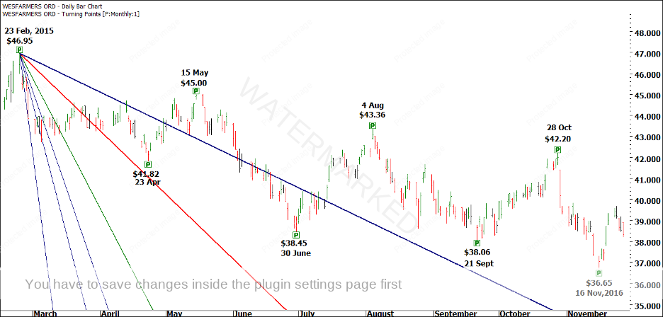
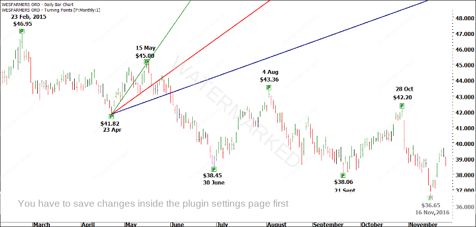
I have used Calendar Days for my chart, and a point size of 0.01. You may remember from the webinar that I use a green line for my 2×1, a red line for my 1×1 and a blue line for my 1×2 angle. You can see from Chart 2 above that a 2×1 angle squared out the top of 28 October, the start of the fourth and final section down. An 8×1 Angle goes close to calling the end of Section 1, as shown in Chart 3 below.
Chart 3

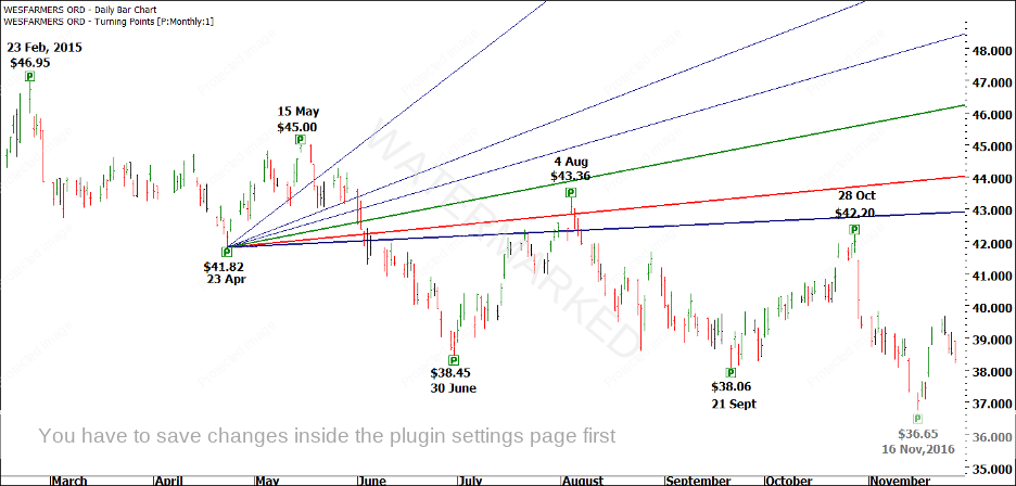
Remember that on 23 April, 2015, you DON’T KNOW that the 2×1 is going to work later. In fact, you would be more likely to use a point size of 0.1, which gives the following hits in Chart 4 below.
Chart 4
You can see that a 4×1 angle helped call the small First Range Out, and the 1×1 and 1×2 angles called the little Double Tops in March and April. From this, you would probably have been expecting the market to fall to the 1×1 line, but it did not – it pulled up short. While Squaring Time and Price was not as clear as you would like in this case, remember that you still had the 200% milestone of the Double Tops, as well as Time by Degrees of 60 degrees, to help you call the 23 April, 2015 low.
In Chart 5, you can see I have run angles UP from the 23 April, 2015 low.
Chart 5
The pullback into the 15 May top was so steep that even an 8×1 angle couldn’t touch it. This is where you need to change point sizes. We will try using 0.1 instead of 0.01, as shown in Chart 6 below. Remember that you will generally need larger point sizes for shorter term moves.
Chart 6
Still nothing! We have tried two different point sizes, and not been able to Square Time and Price. The last thing I would try at this stage would be Trading Days. If we change from a Calendar Day to Trading Day chart, as shown in Chart 7, below, we finally get a scenario where TIME = PRICE.
Chart 7
Now, you may be thinking “Mat’s just running enough angles until he gets lucky and hits something”, but no. Remember from the webinar, we are looking for examples of TIME being EQUAL to PRICE, or Squaring Time and Price. Once you have a run down and a run up like this, you will have a good idea of which angles to use going forward. If you have spent a lot of time on your market, you may already know the best angles to use.
The run from 23 April to 15 May was $3.18 in 16 trading days. Using a calculator, we can see that $3.18 / 16 = 0.19875. In other words, Time is Squaring Out with Price using a 2×1 Trading Day Angle with a point size of 0.1.
As I said during the webinar, you do NOT need to have all of these angles on your chart at the same time. I normally have one or two “permanent” angles that I leave on. The others I can put on when I THINK I have a turn, to see if Time and Price are Square. Remember, we are not using this as a standalone indicator. We are using it to confirm our work with Ranges, and with Time by Degrees. In a later exercise, you will combine all of these techniques together.
We know from our previous work that the 15 May high was 30 degrees from a previous high, and a 62.5% retracement of Section 1. You might like to look at the daily ranges that make up the move from the 23 April low to the May high, to see if you can see any evidence of three sections.
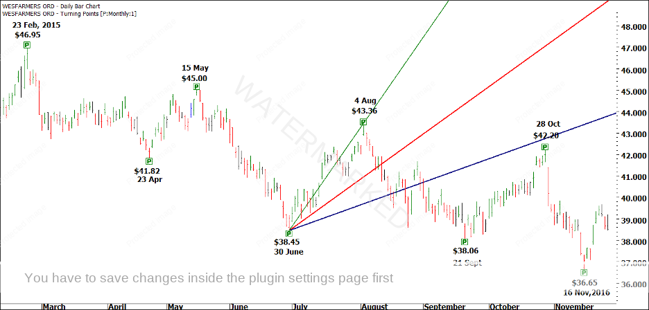
Next, we will run angles down from the 15 May high. We would already be running our First Range Out of $5.13 down from this top. After the difficulties in the previous move, we now know that a point size of 0.1 is worth using, and that Trading Days are worth considering. In Chart 8 below, we will use those settings as a starting point for our angles.
Chart 8
Straight away, you can see that Time and Price square out at the low using a 2×1 Trading Day angle with a point size of 0.1, exactly the same as the previous move. Remember too that this move tied in nicely with the First Range Out – once it had passed 100%, you would be on guard for a change in trend. It might go to 133% or 150% or 200%, but in this case, the market turned just past 125%, after it bounced off the 2×1 angle.
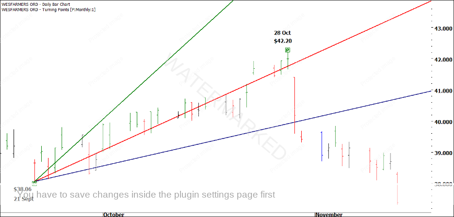
In Chart 9, we can see that the same 2×1 Trading Day Angle using a point size of 0.1 called the next top, which happened to be on the August Seasonal Date. That’s the same angle, three moves in a row.
Chart 9
For the next move down out of the 4 August top, we already know that the First Range Out of $5.13 repeated, and that the low came in around the September Seasonal Date. In this case, the Squaring wasn’t perfect, but a 1×1 Calendar Day Angle was very close to the low, as shown in Chart 10 below.
Chart 10
This is an example of wearing the market like a loose garment. It is not perfect, but it is very close. The key thing is that we have a 100% repeat of the First Range Out on a Seasonal Date, with an almost perfect squaring. That is enough for me.
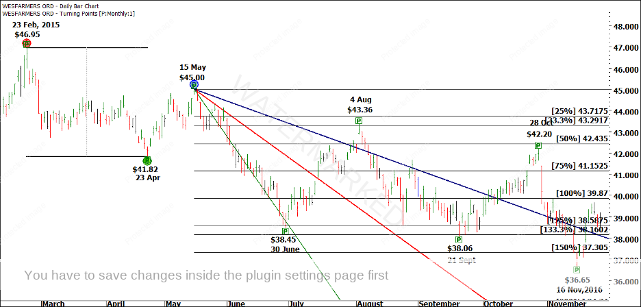
Chart 11
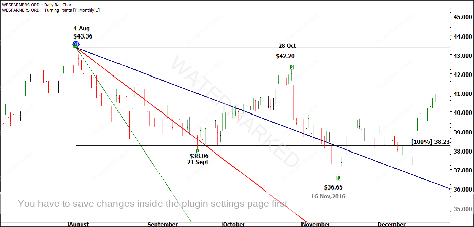
We know that a 2×1 Calendar Day angle down from the 23 February, 2015 high called the 28 October top. You can also see that a 1×1 from the September low came close to the top, in Chart 11, above.
That leaves us with the final run down. We already know that the last run down was quite steep, and our angles confirm this for us. It was a 4×1 Trading Day angle that called the low, an angle running at twice the speed, or twice the pitch of the 2×1 Trading Day angles we have seen working previously on the market.
Chart 12

You can see that Squaring Time and Price is a very valuable addition to your trading arsenal. The lessons in this webinar, are actually just the beginning. In the Ultimate Gann Course, David introduces you to the concept of Speed Angles, while in the Master Forecasting Course, David introduces you to other types of angles, and other places to run them from. Students with these courses may like to do some further work on this Wesfarmers example. They may just find an additional angle that locks in the 16 November, 2015 low perfectly.